Part 4: Comprehensive CFD Software Packages; Siemens STAR CCM+ Vs. ANSYS Fluent
Comprehensive Multiphysics Simulation Packages – La Crème de la Crème

Batman versus Superman, Magic versus Bird, Yankees versus Red Sox, Microsoft versus Apple, Ferrari versus Lamborghini, Coke versus Pepsi… you get the point. The world is full of great rivalries at the top tiers of competition. It is no different in the world of CFD simulation where Fluent and STAR-CCM+, and before that STAR-CD, have been battling for market leadership for over 20 years. And while one’s preference for Magic or Bird may be an opinion, a discussion of their claims to being called the best at what they do is healthy. We hope the following discussion of Fluent and STAR-CCM+ is helpful to everyone who will take the time to read it (spoiler alert: it’s really long) but expect it will be especially so for those users with some CFD experience who are looking into upgrading to a comprehensive CFD software package.
And while one’s preference may be for Magic or Bird, Iphone or Android, a discussion of their merits and faults is healthy.
Example #1: Siemens Simcenter STAR-CCM+
In full disclosure, Resolved Analytics became a Siemens Channel Partner in 2020 supporting sales of STAR-CCM+ after initially posting this series.
STAR-CCM+, and before that STAR-CD, was originally developed by researchers in Imperial College’s CFD research group in the late 1980s. In time, these contributors and others founded the company known as CD-Adapco with the aim to bring CFD to the masses. At the time of its acquisition by Siemens AG in 2016, CD-Adapco’s annual revenue was around $200M and was growing at a CAGR of 12%. Their customer base at the time was around 3,200 at an average revenue of $65,000 per customer. STAR-CCM+ is the leading provider of Multiphysics to the automotive industry which contributed 52% of CD-Adapco’s revenue at the time. STAR-CCM+ is now a Computational Aided Engineering (CAE) solution for solving multidisciplinary problems in both fluid and solid continuum mechanics within a single integrated user interface.
Basic Interface & Workflow
STAR-CCM+ offers a very clean, modern interface; a result of the complete overhaul of the original STAR-CD software that took place in 2005. STAR-CCM+ is available for both Linux and Windows operating systems without major differences to the interface. The user can access all pre-processing, simulation, and post-processing tasks from within this single interface. Batch commands for all processes can also be issued through the command line or through scripts written in Java.
STAR-CCM+ User Interface
Tools are organized to streamline workflow from CAD creation or import, through meshing, setup, simulation and processing of results. Workflow organization is from top to bottom in the “Simulation” tree on the left, while system level commands are accessed via the toolbar at the top. Geometries are initiated by CAD import (.stl, .x_b, .step, .iges), by CAD creation using the built-in CAD modeling tools, or by mesh import from 3rd party tools. Direct import of solid models from leading 3D modeling programs including SolidWorks, Inventor, NX, Pro/ENGINEER, Rhino and CATIA is also possible with the additional purchase of a translator plugin. Once imported, geometries are categorized as “parts” and “part-based operations” are encouraged by the STAR-CCM+ workflow. That is, all future operations, such as applying surface meshes or specifying boundary conditions, are performed with reference to the original part, rather than continuum volume regions (meshes) created in subsequent steps. The parts-based workflow ensures that most of the simulation setup will not need to be repeated when replacing parts with modified geometries.
Physics Modeling Capabilities
STAR-CCM+ contains a wide range of physics models and methods for the simulation of single- and multi-phase fluid flow, heat transfer, turbulence, solid stress, dynamic fluid body interaction, aeroacoustics, and related phenomena. New features are continually introduced through regular releases. Core physics modeling capabilities include inviscid, laminar or turbulent flows, Newtonian or non-Newtonian viscosities, incompressible or compressible flows, multi-component mixtures, multi-phase mixtures, porous interfaces or volumes, passive scalars, steady or unsteady flows, ideal or real gas law equations of state, conduction, convection, radiation, reacting flows and motion.
STAR-CCM+ comes with a database of common materials in categories of solid, liquid, gas, and electrochemical species and a wide range of turbulence modeling options including RANS models, Reynolds Stress Transport models, detached and large eddy simulation models, and laminar-to-turbulence transition models. STAR-CCM+ leads the industry in multi-phase physics modeling capabilities including Eulerian Multiphase flows (gas, liquid or solid), granular phase models, population balance models (bubble size distributions), wall and bulk boiling models, Volume of Fluid (VOF) based surface tracking models, fluid film models, dispersed and mixture multiphase models, Lagrangian phase models, and Discrete Element Modeling (DEM) models for large numbers of interacting discrete objects. Both moving reference frames and moving and deforming meshes can be used to capture the effects of fluid or solid motions on one another. Motion can either be user-defined or defined by Dynamic Fluid Body Interaction (DFBI). Reaction chemistry models include the ability to model solid, liquid or gaseous fuels, premixed or non-premixed combustion, surface reactions, particle reactions and coal combustion and polymerization. Combustion models include flamelet models and reacting species transport models such as Eddy Break-Up Models. Complex chemistry can be defined through user input or through STAR-CCM+ interface with 3rd party tools such as Chemkin. Electrochemistry, plasma dynamics, electromagnetism, aeroacoustics, and computational rheology models are also included.
A finite element solver has been added recently that allows basic solid mechanics modeling, including static, dynamic and quasi-static analyses, linear or non-linear geometries, hexahedra, tetrahedra, wedge and pyramid type elements, isotropic and anisotropic linear elastic materials, and a variety of loads and constraints on points, surfaces and bodies.
The software is distributed with a full suite of verification and validation test cases that can be analyzed for both physics model validation and software/hardware implementation verification.
CAD Cleanup and Meshing
STAR-CCM+ makes the process of importing, repairing, defining and meshing your CAD parts about as painless as it can be. At its most basic, cleanup to meshing consists of associating part level volumes and surfaces to the appropriate physics, volume meshes and boundary conditions which will be the basis of the numerical simulation. Many part-based operations are available, such as part transformations or Boolean operations. The choice of whether to perform such operations within your typical 3D solid modeling software or within STAR-CCM+ is based on user preference.

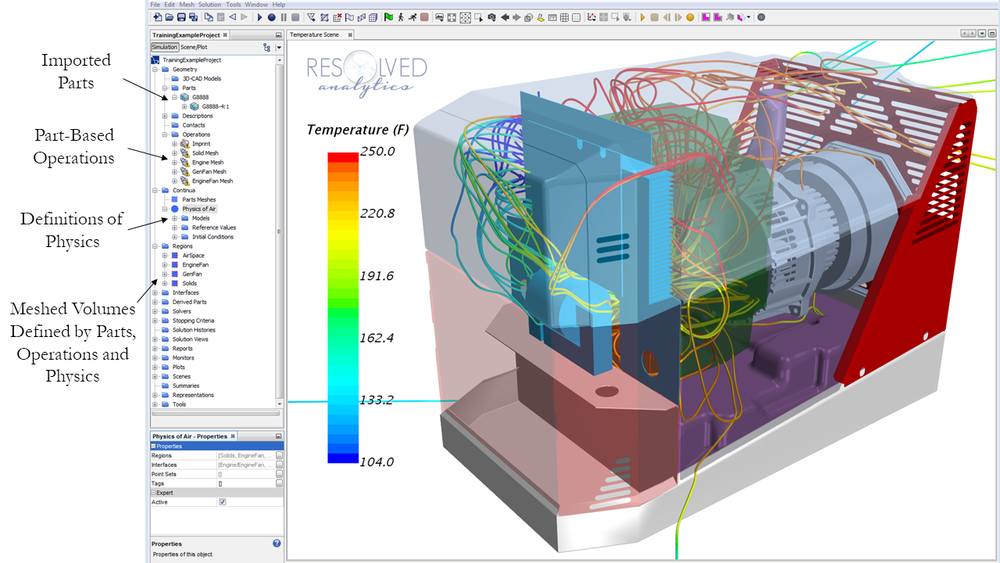
STAR-CCM+ Parts-Based Workflow
The screen shot here depicts a few pre-processing elements for simulating the natural convection driven cooling of an electronics enclosure, including the conjugate heat transfer through the walls of the enclosure. Two parts have been imported, a box representing the air surrounding the enclosure and the enclosure itself. The far field air boundaries, shown transparently, which will be assigned non-wall boundary conditions, have been split from the remainder of the air surfaces before a Boolean Subtract is performed subtracting the latter part from the former. This operation defines a new part, called here “AirMinusSolids” which is then promoted to a “Region” and assigned to the relevant physics continuum. The same is done for the “Enclosure” Part. Mesh operations are then defined for each Part/Region association.
For those times when 3D solid models are less than ideal for CFD model workflows, STAR-CCM+ provides several tools to help in diagnosing and repairing geometry. A useful option that can be turned on when importing geometry is to “Check and Repair Invalid Bodies” which automatically resolves some simple but common issues that produce invalid geometries, such as very close, but non-coincident surfaces, holes and pierced faces. Another tool that comes in handy when importing parts with very small or problematic features, such as holes or intersections, that are unimportant to the physics of interest, is the “surface wrapper” tool. The surface wrapper tool provides a closed, manifold, non-intersecting surface when starting from a poor-quality CAD model. The resulting part is then used to create a volume mesh associated with a physics continuum in the same manner as typical imported parts.
STAR-CCM+ makes the process of importing, repairing, defining and meshing your CAD parts about as painless as it can conceivably be.
Another process which STAR-CCM+ handles particularly well is mesh generation. Typically, parts surfaces are first remeshed in order to improve the quality of the final volume mesh and to specify geometries where higher mesh densities are needed. Volume meshes can be applied with a wonderful array of controls and features and can be performed in either serial or parallel modes, granted the user has access to parallel hardware and software license resources. The three primary mesh model types are tetrahedral, polyhedral and trimmed (hexahedral). Tetrahedral meshes, generally, are fast and reliable to process, allowing for complex geometries to be meshed with fewer errors, but result in lower accuracy in results. Polyhedral meshes, it’s claimed, provide a balanced solution for complex mesh generation problems while having higher accuracy than tetrahedral meshes. Trimmed cell meshes produce the highest quality grid by utilizing predominantly hexahedral volumes with minimal skewness and alignment with flow.

STAR-CCM+ high density prismatic meshing of boundary layers
Prismatic near-wall layers can be included with all three types of mesh by including the prism meshing model as part of the volume meshing process (as shown in the following figure). Typical surface and volume mesh controls include the default cell size, the minimum and maximum cell sizes, the cell growth rate, prism layer thickness, number of prism layers, and allowable quality metrics.
Simulation
STAR-CCM+ employs both segregated and coupled finite volume flow solvers as well as the finite element solid stress solver mentioned previously. In the segregated flow solver, the relevant equations are solved in an uncoupled manner and momentum and continuity equation solutions are linked via a predictor-corrector approach. Solutions are updated at each iteration based on the SIMPLE algorithm developed by Professor Spalding at Imperial College. For both all relevant equation solvers, advanced controls for under-relaxation factors and algebraic multigrid cycles are available.
In the coupled flow solver, the relevant equations are solved simultaneously using a pseudo-time approach. This approach is advantageous for flows with dominant source terms, such as rotational or buoyancy driven flows, as well as highly compressible flows. The coupled implicit solver controls the solution update for implicit spatial integration in both steady and unsteady analyses using a coupled algebraic multigrid method. The coupled explicit solver can be used for explicit integration using a Runge-Kutta multi-stage scheme if desired. The segregated solver is generally preferred for incompressible or mildly compressible flows due to its numerical and data storage efficiencies compared to the coupled solvers.
With each new release, Siemens provides a verification suite of test cases that come from the SIMCENTER STAR-CCM+ quality-assurance process. This extensive process includes an internal test system that is known as STAR-Test, which is used continuously for the development and release builds of the software. With this suite of cases, the user has the opportunity to verify that the software received is able to reproduce the same results on the platform you are using (verification) while also providing an understanding of the accuracy to be expected when modeling specific physics use cases (validation). Each case comes with its own documentation describing the experimental setup to which it was compared as well as the relative accuracy of the simulation result. To the best of our knowledge, STAR-CCM+ is the only multiphysics simulation tool that has achieved ASME Nuclear Quality Assurance – 1 compliance.
Post-Processing
STAR-CCM+ provides perhaps the most striking and intuitive flow visualization techniques among all leading CFD software packages and which are comparatively easy to use. We rate the inherent capabilities of STAR-CCM+ on par with the capabilities of leading stand-alone visualization packages such as FieldView. Foremost, it is possible to watch a flow field evolve as the simulation iterates, allowing the user to change parameters and immediately see the effects of those changes upon the simulation. This interactive feedback allows for the dynamic supervision and control of the simulation as well as insight into the physical aspects of the simulation. Further, since visualization in STAR-CCM+ utilizes a client-server environment, the bulk of data processing takes place on the server process. Only the lightweight graphics data is sent to the client, allowing for a massively parallel simulation to be visualized from a client workstation.
STAR-CCM+ provides perhaps the most striking and intuitive flow visualization techniques among all leading CFD software packages and which are comparatively easy to use.
Animation from CFD Simulation of a Water Pump utilizing the Volume Rendering Tools within STAR-CCM+ to Best Visualize the Downstream Wake
In STAR-CCM+, all of the common CFD displayers are available including scalar, vector and streamline displayers that can be shown on surfaces or volumes. Several specialized tools, though, really make STAR-CCM+ standout from the competition. For one, a tool known as volume rendering can be used to display semitransparent, volumetric objects that are defined in a 3D domain. These resampled volumes, or voxels, allow the user to “look inside the flow” by assigning opacity to the contoured surfaces that make up a volume-based definition of a quantity of interest. Combining volume rendering with the slick animation recording capabilities of STAR-CCM+ allows the production of realistic visualizations of time-dependent phenomenon, such as the simulation of a water pump shown below.
Speaking of time-dependent simulations, STAR-CCM+ allows for saving selected data while a simulation is running through what is known as a solution history file. After the simulation completes, the solution history file is loaded and the user can query through its states for post-processing. In addition to the solution data, each simulation history file can contain a copy of the volume mesh, the standalone boundary surfaces, or both. Recording the relatively light weight simulation history file at your needed temporal resolution allows the user to create after-the-fact animations of whatever visualization they desire, without needing to intuit ahead of time the most appealing and insightful animation to be recorded in the form of static graphics files.
Two new visualization capabilities that we will be excited to work with moving forward are the STAR-CCM+ Virtual Reality (VR) technology and screenplay functionality. VR delivers exactly what it sounds like it would deliver, the opportunity to move around inside a simulation result which has the potential to provide more useful insight. Screenplay functionality is like a typical animation on steroids. With screenplays, the animation recording is no longer constrained by a single visualization and, instead, visualizations can dynamically change throughout the recording. Properties such as the quantities being visualized, the viewing angle, object transparencies, and so on can be varied as the recording progresses, as well as synchronized with the time-stepping of time-dependent data through the simulation history files mentioned previously. We collected a number of the most impressive STAR-CCM+ visualizations we’ve seen in the video below.
A Compilation of STAR-CCM+ CFD and Multiphysics Animations from 2019
But post-processing is more than just pretty pictures. We really find the depth of the post-processing quantification tools available within STAR-CCM+ to be extremely useful. If you can think of it, it can probably be output and/or recorded from STAR-CCM+ without a significant amount of effort. Most of the quantities you’ll wish to record start as “reports”. Reports can take on a wide range of attributes, while most are statistical in nature, such as averages, minima and maxima, integrals, and standard deviations. These statistical measures can be extracted over points or sets of points that you can easily create, or predefined surfaces or volumes. Several useful physics-based reports are baked in, including force, heat transfer, pressure drop, and mass flow reports, along with many others. Reports can quickly and easily be turned into monitors which track the report value over iterations or time steps, and these monitors can in turn be converted with a single mouse click into xy-plots. Furthermore, such xy-plots can then be used as annotations on flow visualizations. Oftentimes we find that statistical monitors can serve as more effective convergence criteria than the typical iterative numerical error residuals, and they are easily used in this fashion. Heat maps and histograms are also natively available.
If you can dream it up, it can probably simulated and visualized in STAR-CCM+ without superhuman effort.
Summary
We don’t find many flaws with Siemens STAR-CCM+. In fact, it makes our lives as consulting engineers easier everyday by providing a full-suite of multi-physics capabilities, a streamlined workflow within a modern java based interface, best-in-class meshing capabilities and insightful, meaningful and impressive post-processing without the prerequisite of obtaining a Ph. D. in programming. As with all things, much is in the eye of the beholder, but we believe in the power of this software so much that we’ve partnered with Siemens Digital Industries Software to offer STAR-CCM+ to our customers. If you’d like pricing or a more information on its capabilities you can contact us here.
Pros: powerful, efficient and validated numerical methods, full suite of physics and multiphysics capabilities, streamlined workflow and ease-of-use, post-processing
Cons : still looking
Example #2: ANSYS Fluent
We grew up in the South where the word “coke” was used instead of “soda” or “soft drink.” Coca-Cola wasn’t all we had (obviously, there is always sweet tea), it was just that Coke seemed to dominate the regional market in such a manner that all other sodas were simply referred to as “cokes”. Although ANSYS Fluent doesn’t quite have the same name recognition whereby “CFD” can be replaced with “Fluent,” there are some parallels. As one of today’s leading CFD software packages, Fluent has built a strong reputation in the field and is well known, well respected, and well accepted. It is so common, that we frequently get requests from customers and potential customers for our .cas (or “case”) files, which are native Fluent files, assuming that we use Fluent in our work.
Fluent’s history goes back to the early 1980’s when a New Hampshire based company called Creare collaborated with a research group at Sheffield University in the UK to create a CFD software product for a wide range of engineering applications. In 1988, Fluent, Inc. was formed as a result of the collaboration, and in 2006, ANSYS purchased the corporation.
Fast forward to today, where technology has advanced by leaps and bounds, and there are numerous well established CFD packages out there. Is Fluent among the best available commercial CFD software packages? We’ll try to answer this question by reviewing the latest Fluent offering, version 2019 R2, to find out about its ease of use, meshing, speed, ability to automate and customize, post-processing, customer support and accuracy.
Package Contents
To get up and running with Fluent, ANSYS offers several packages (or bundles) that include Fluent in addition to other support software. The “CFD Premium Bundle” includes Fluent, Workbench (a project-style wrapper that manages multiple software tools), SpaceClaim (a CAD tool which is now a stand-alone software), Ensight (a post-processing software package), CFX (another CFD solver) as well as CFD-Post (a post-processing tool that was built for CFX but works nicely with Fluent results as well).
Although Fluent can be used in either Windows or Linux-based versions, it should be noted that SpaceClaim is currently only available for Windows operating systems.
Basic Interface & Workflow
Currently, our preference is to use a stand-alone CAD package for initial geometry creation, such as SolidWorks or AutoDesk Inventor. This geometry is then brought into SpaceClaim in order to separate and label parts and boundaries as well as create any needed mesh refinement zones (“bodies of influence”). Next, the SpaceClaim geometry file is imported to Fluent for pre-processing, meshing, and running the simulation. If you haven’t used Fluent in a while, you may be wondering what happened to Design Modeler and ANSYS Mesher, two Workbench tools that were required steps prior to generating a Fluent mesh. With the new “Watertight Workflow”, one only needs to use SpaceClaim (in place of Design Modeler) and then bring the geometry directly into Fluent for native meshing. While Workbench did have its advantages, especially when coupling geometry modifications and multi-physics applications where fluids solvers (Fluent/CFX) are coupled with solid/FEA solvers all in one environment, we consider the ability to bypass Workbench a very good thing.

Fluent User Interface with “Setup” tree on left, Main viewing window on right, and “Console” along bottom
The main Fluent interface is shown below and will look familiar to many readers, as it has not changed significantly in recent updates. Boundary conditions, fluid types/properties, solver settings, stopping criteria, etc. all must be input before launching the simulation via the “Setup” tree on the left-hand side. Upon clicking any of the tree items, “the task page” shows more details. The geometry, or any plot or contour if a solution is loaded, is viewed through the main window on the right. For legacy users, the text-user-interface (TUI) allows for keyboard command input in the “Console” window at the bottom. This is also where residuals and warnings will print out during simulation. If you need to locate something, the ribbon across the top allows for quick access to most of the items in the tree.
Once all of the boundary conditions, physics settings and solver settings are ready, the simulation can either be launched directly from within Fluent or via a batch or job submit script (this does require the case and data files to be written). Once complete, the results can be analyzed either from within Fluent, via CFD-Post, or via Ensight.
Physics Modeling Capabilities
As expected, a multitude of material properties and physics options are available within Fluent, including RANS steady-state, transient, segregated and coupled solvers, laminar, turbulent, and transitional flow solvers, single-phase or multiphase techniques (including phase changing), mesh motion, energy sources and sinks, chemical reactions, passive scalars/tracers, and more. LES and DES solvers are also built in. If there is some sort of physics phenomena that isn’t built in and available, Fluent supports the use of user codes called UDF’s (User Defined Functions), which are fully customizable scripts that allow you to tap or “hook” into the flow variables in order to model the physics/behavior at each computational cell.

Demonstration of Fluent Volume-of-Fluid to Discrete Phase Model
Although we haven’t had time to fully investigate, we are really excited about the new GEKO turbulence model by Dr. Florian Menter’s group that is now included within Fluent and can be described as a hybrid between two of the most popular RANS two-equation models out there: K-Omega SST and K-Epsilon Realizable.
Another promising feature is the new hybrid Volume-of-Fluid (VOF) to Discrete Phase Model (DPM) that is used for spray nozzle simulations. This new VOF-to-DPM multiphase approach converts bulk liquid tracked via the VOF model into blobs and droplets that are tracked by the DPM/Lagrangian technique. The figure on the right, provided by ANSYS, gives the reader the idea of how this new model functions.
CAD Cleanup and Meshing
As mentioned above, the new methodology within Fluent is being called the “Watertight Workflow”. A screenshot of the workflow “tree” in Fluent is shown below. This tree structure guides you from top to bottom as you import geometry, add meshing parameters, label boundaries and zones/regions, and create surface and volume meshes. Compared to the previous native Fluent meshing, this recent advancement is a huge upgrade in the user-friendly department. Note that the “Import Geometry” feature allows for direct import of universal CAD files such as Parasolid, albeit with the purchase of additional license features. Instead, we use SpaceClaim to preprocess solid model geometries that can then be exported to Fluent directly. SpaceClaim can import universal and native CAD files including Parasolid and SolidWorks formats.

Fluent Watertight Geometry Workflow Tree
The key feature that has been added here is that the user can now import solid geometry and then, within Fluent, generate the interior “fluid space” for running the CFD simulation. This is all done within the Watertight Workflow tree “Enclose Fluid Regions” functionality. In theory, one could create geometries solely within the ANSYS package and there would be no need for an external CAD package. However, we continue to find it more convenient to generate fluid domains within an external CAD package before importing into SpaceClaim/Fluent, which is also a perfectly acceptable technique. It should be noted that SpaceClaim itself is a fully functioning 3D CAD tool. You can create geometries from scratch, as you can in any other well-known CAD package, though the interface does take some getting used to, as there is no CAD “tree” of operations that details how the 3D parts have been built. Using a direct modeling approach, SpaceClaim requires a different mindset than the more common parametric modeling approach of SolidWorks and Inventor —bodies and faces are stretched and pulled using the mouse rather than setting up a sketch first and then extruding/cutting via feature functions with specified dimensions.

Fluent View of Automatically Displayed “Cut Mesh”
Once the Watertight Workflow is complete and the mesh has been created, it’s time to set up the CFD simulation parameters. At this point, the user saves the generated mesh via writing out the .msh file. It is a good idea in general to write/save often, especially once all physics/settings have been setup via writing out a .cas file just “in case” things go downhill (pun intended).
The meshing within Fluent is where the latest versions really shine. The process is now straightforward, and the workflow guides the user though the remaining effort. The volume meshing options are tetrahedral, hexcore, polyhedral, and poly-hexcore. One feature we love is the “preview” of the mesh size that allows the user to see how small/large the computation cells will be before anything is meshed. This can save a lot of time that could otherwise be wasted by meshing a geometry with too coarse or too fine of a grid. We also like the automatic “cut view” of the resulting mesh upon completion, as shown below.

Fluent Poly-hexcore mesh
Another update to the native Fluent mesher in recent versions is the new Mosaic meshing technology, also called “poly-hexcore”. This mesher creates a hybrid hexahedral/polyhedral mesh where flow-aligned hexahedral cells are created in the bulk flow zones with wall-aligned polyhedral cells and boundary layer cells (“inflation layers”) are utilized near walls. According to Fluent’s literature, this mesh type is showing an improvement in total cell counts for similar (or boosted) accuracy when compared to polyhedral alone (which increases speed). We were able to easily create a poly-hexcore mesh during testing for an internal flow geometry. Compared to the polyhedral mesh we generated with the same min/max cells size settings, the poly-hexcore mesh had ~10% fewer cells in total. We also noted an improvement in meshing time from 3 minutes (on 4 cores) for the poly-hexcore compared to ~13.5 minutes for the corresponding all-polyhedra mesh. This is quite a speedup (~4.5x) and could save major time for generating larger, more complex meshes.
In addition, as expected for a software of this type, parallel meshing is available, which improves meshing times by utilizing more available processors.
Simulation
Fluent includes a wide range of numerical solvers, both segregated/SIMPLE and pressure-velocity coupled for high-speed cases. Fluent is fully parallelizable if you have the available cores or can run your cases in the cloud. Jobs can be run locally through the GUI that was used to set up the case or they can be run in batch mode from a command line or job submit script. Cases can be run in Linux even if they were pre-processed and set up in Windows, or vice-versa. Flow-field data (full mesh or at certain pre-set monitor points/locations) can be auto-saved/exported during the simulation, which is especially handy for transient cases and debugging.
One newish feature that we like is the ability to monitor your case with a “report” value that is set up prior to launch. You can report out pressure drop across certain planes/boundaries for example, at each iteration if needed. This can also be plotted on the fly during simulations, and convergence criteria can be created based on these custom reports. We know these features are available in other software packages, and they are a welcome addition to recent Fluent releases.
Although we haven’t tested it, ANSYS is touting some pretty impressive performance improvements via the use of GPU processors for Fluent computations. We imagine that actual performance improvements will vary quite a bit with specific case setups.
Another new feature is the ability to create user “field functions” within the GUI and can be based on any existing flow field parameters such as pressure, density, etc. These can, and likely will, take the place of the more complex User Defined Functions (UDFs) which require a complied code/script written in the C programming language.
Lastly, ANSYS maintains a suite of test cases which are run on the software prior to each release. The purpose of this testing is to allow the user to verify that the software performs according to documentation and to provide the user with confidence that it can adequately solve various physics problems within tolerable levels of accuracy. We strongly recommend for you to check out the list to see if your use case is covered.
Post-Processing

Fluent post-processing example
Once the simulation is complete, there are several options for post processing the results. The general CFD post processing capabilities are present within Fluent, such as contours, streamlines, vectors, and analyzing data via XY plots. Another option is CFD-Post, which also provides similar features. For transient cases, CFD-Post may be easier to work with, but we think it really just comes down to user preference. We do like that you can save off a “state” file in CFD-Post (.cst). This is handy if you have a lot of cases that were run for the same geometry (or similar geometry) and you want to ensure all plots are consistent. The state file can first be loaded, and then the results (data files) for each case can be imported into the “state.” If streamlines, contours, and XY plots were created, they do not have to be re-made for each data file, as they are stored in the state file.
Ensight, which is a new ANSYS acquisition, is an entirely different option for post processing. Unfortunately, we are not familiar with it but have seen some exceptional videos/images online that showcase what can be done. It appears to be able to show both solid FEA model results as well as fluid CFD cases and can be quite impressive for analyzing and animating fluid-body-interaction data. This powerful tool comes with Fluent and seems worth your time to investigate if you haven’t already.
Summary
With a strong history in CFD, cutting edge and continuous upgrades to the code base and capabilities, a reputation for providing accurate and validated results for numerous flow cases/types, a stout user base and community, and dedicated customer support with a vast array of online resources and webinars, overall Fluent is a strong multi-physics software platform. Recently added capabilities have greatly increased its ease of its.
Pros: powerful, efficient and validated numerical methods, full suite of physics and multiphysics capabilities
Cons: requirement for standalone software for pre-processing (SpaceClaim) and superior post-processing (Ensight), cost