Part 3: Semi-Comprehensive CFD Software
How Has CFD Market Consolidation Changed Your Software Options?
Since the original publication of this review, the CFD landscape has shifted from a field of independent specialists to an ecosystem dominated by three primary conglomerates: Siemens, Ansys (now Synopsys), and Cadence Design Systems. Most notably, Numeca International and Future Facilities (6SigmaET) have been integrated into the Cadence Fidelity platform, while Altair’s specialized solvers (AcuSolve and nanoFluidX) have joined the Siemens Simcenter portfolio. These acquisitions mean that "Semi-Comprehensive" tools are increasingly being rebranded as specialized solvers within larger, end-to-end multiphysics environments.
Key Acquisition Tracking (2021–2026):
Cadence Fidelity CFD: Now includes the technologies formerly known as Numeca, Pointwise, and 6SigmaET.
Siemens Simcenter: Recently expanded to include Altair’s entire simulation suite, consolidating the industry’s leading particle-based and LBM solvers.
Synopsys-Ansys: The 2025 merger of these two giants has unified electronic design automation (EDA) with the world’s largest CFD install base (Fluent/CFX). For a full review of Ansys Fluent and STAR-CCM+ as comprehensive solvers, see Part 4 of this series.
Pure-Play Independents: COMSOL and Convergent Science (CONVERGE) remain the primary independent holdouts, maintaining their focus on research-driven and autonomous-meshing niches respectively.
2026 CFD Market Analysis: Cloud Scalability, GPU Acceleration, and Licensing Models
A Note on "On-Demand" Myths:
While many cloud providers advertise CFD software "on-demand," there is a critical distinction between hardware and software billing that can lead to unexpected project costs. Companies like Cadence and Convergent Science now offer true "Consumption-Based" licensing, where you pay for both the server and the software by the hour. In contrast, COMSOL remains a "Bring Your Own License" (BYOL) platform; while you can run it on-demand cloud hardware, you must typically own a pre-paid annual or perpetual Floating Network License (FNL) to do so. Understanding these nuances is key to selecting a solver that aligns with your specific project timeline and budget.
| Software | True On-Demand? | GPU Ready? | Cloud Strategy |
|---|---|---|---|
| Cadence Fidelity (Formerly Numeca) |
Yes Full SaaS / OnCloud Tokens |
Yes Native CUDA Solvers |
Very High Native SaaS Environment |
| CONVERGE CFD | Yes Pay-as-you-go via Horizon |
Partial Newly added in v5.0 |
High HPC Cloud Platform |
| COMSOL | No BYOL (Annual License Required) |
No CPU Matrix-Based Solvers |
Low Partner-managed Hardware |
What Makes a CFD Tool 'Semi-Comprehensive' and Why Does It Matter?
These tools try to do everything — and come remarkably close — but knowing where they fall short is what separates a good simulation from a costly one.
Key Takeaways:
• Semi-comprehensive tools (COMSOL, CONVERGE, Cadence Fidelity) dominate specific niches but fall short of comprehensive platforms for general industrial CFD.
• COMSOL is the strongest choice for coupled multiphysics with user-defined equations — especially in academic and R&D settings.
• CONVERGE is the industry standard for internal combustion engine and reacting flow simulation.
• These tools carry premium pricing comparable to comprehensive platforms, without the same breadth.
• The key question: does your problem sit squarely in the tool's niche? If yes, it is likely the best choice. If not, look at Part 4, Comprehensive CFD Software.
In our original post, we defined the highest-performing CFD software class as “Comprehensive”. The following is our not-so-scientific list of criteria we used for classifying software packages as “Comprehensive” or not.
The capability to import complex 3d solid and surface geometries from diverse sources
An all-in-one workflow, including pre-processing, simulation and post-processing
Broad multi-physics simulation capabilities
Efficient data architectures, numerical methods and utilization of diverse hardware and software configurations
Vendor initiated verification and validation of physics and numerical methods
Limited requirements for user-coding and/or command line operations
In this section, we’re discussing software packages that strive to be comprehensive, multi-physics tools but, in our opinion, fall just a little short in some respect. There are many available CFD software packages that could be described as semi-comprehensive, and we couldn’t possibly review them all and still get any real work done. So here, we are focusing on three software packages in this category based on their large user base and/or their potential to become comprehensive: COMSOL Multiphysics, CONVERGE CFD, and Cadence Fidelity (Formerly Numeca OMNIS). Some of the other software packages in this semi-comprehensive category that we would have liked to review if we had more time include Siemens' Altair AcuSolve, Flow Science FLOW-3D, Cadence's SC/Tetra (formerly MSC), and the cloud-native SimScale.
All three of the tools discussed here have the potential to be extremely valuable in the right context.
Example #1: COMSOL Multiphysics: The Research Platform That Is Finally Becoming an Engineering Tool

COMSOL was established in July, 1986 with a headquarters in Stockholm, Sweden. The founders were former doctoral students of professor Germund Dahlquist at KTH and originally partnered with US based Mathworks as a European distributor of MATLAB. During this period COMSOL developed its own software known as FEMLAB that expanded the capabilities of MATLAB in solving partial differential equations. At first, FEMLAB was dependent upon MATLAB engines, but by the time the two companies parted ways in 2004, COMSOL had developed their own finite-element based meshing and solving routines. As with MATLAB, the software was considered a platform with additionally available toolbox components built for creating and executing simulations in various physics domains. Early successes were primarily with universities and research labs, including close cooperation with Chalmers and Stanford among others.
In 2005 FEMLAB became known as COMSOL Multiphysics (COMSOL). Utilizing a graphical user interface (GUI) combined with a “MATLAB like” programming interface, researchers could customize an analysis utilizing the FEMLAB tools to solve their specific physics application in multi-dimensions as never before. COMSOL very neatly filled the gap between MATLAB’s lack of spatial discretization sophistication and the more widely available GUI based, spatial solvers, such as ANSYS, that lacked an easy-to-use programmatic interface allowing application of general solution routines to researcher specific differential equations and boundary conditions.
Although recently marketed as a general-purpose engineering tool, COMSOL has traditionally been used more by researchers than by engineers. COMSOL, though, has been working to change this, attempting to thread the needle between increasing ease-of-use for engineers without alienating their historically research-oriented user base. As of 2026, the release of version 6.4 has solidified this shift by integrating AI-assisted modeling and large language model (LLM) support, which helps non-experts navigate complex physics setups. Furthermore, the introduction of the Model Manager and the COMSOL Compiler has successfully pushed the software onto the factory floor and into design departments, allowing experts to deploy simplified "apps" to a much broader engineering audience.
Basic Interface & Workflow

COMSOL Multiphysics Graphical User Interface
Lucky for you, at Resolved Analytics we are all about doing the hard work so you don’t have to. Let’s get started with a look at the COMSOL interface and workflow. The COMSOL recommended first step is to use the “model wizard” option to specify the nature of the multi-physics problem that you wish to simulate, such as whether the problem is 2-D or 3-D in nature, what physics will be included, and whether the problem is steady-state or time-dependent. As of 2026, the Model Wizard has been augmented with an LLM-based Chatbot window. This allows users to describe their physics intent in natural language, which the software then translates into a preliminary Model Tree structure—a major step forward in making the expert-level tool more accessible to engineers. After completing this step, the user enters the “model builder” portion of the workflow.
As with most multiphysics simulation software, geometry is first either created or imported. The COMSOL GUI includes a set of computer-assisted design (CAD) tools for geometry modeling in 1-D, 2-D, and 3-D, but in most engineering cases, it is more efficient to import surface files from existing 3D solid models or create new geometry using the more sophisticated tools available in your company’s 3D solid modeling software of choice. With version 6.4, the CAD Import Module now includes a selective assembly tree preview and automatic "surrounding domain" creation, which automates the tedious task of defining fluid regions around complex solid parts. The model explorer on the left-hand side of the “model builder” window displays the menu items that will be subsequently used to define simulation parameters, boundary conditions, and so on. Furthermore, the interface now includes the Model Manager as a core workflow pillar. This provides integrated version control and data management directly within the GUI, ensuring that multi-user teams can track changes to the physics and geometry without the need for external file-management systems.

COMSOL Multiphysics Product Suite
Physics Modeling Capabilities
COMSOL adopted and remains committed to the MATLAB model whereby the licensee purchases the platform and additional “toolboxes”, or modules, as needed to fit their project requirements. These toolboxes contain what you’ll need to setup and execute your domain-specific problems. Originally consisting of chemical engineering, electromagnetics and structural mechanics modules, the list has now grown to over 50 specialized modules as of the 2026 release of Version 6.4. Check out the product suite chart from an older version here. Within the CFD module, COMSOL offers a variety of multiphase models including the level-set method for free surface interface tracking, a Eulerian-Eulerian dispersed phase model, and a Lagrangian particle tracking model. A significant addition in the current version is the Granular Flow Module, which provides dedicated physics for simulating the behavior of dense particulate systems, such as those found in pharmaceutical and mining applications. Fluid structure interaction is possible using either one-way or two-way coupled procedures. All types of flow rheology can be simulated including Newtonian, viscoelastic and other non-Newtonian behavior, as well as flow within porous media. There are also a number of turbulence wall models and turbulence subgrid-scale models available, including the recently added v2-f turbulence wall model. as well as modernized Large Eddy Simulation (LES) and Detached Eddy Simulation (DES) formulations. Crucially, in 2026, COMSOL has introduced native GPU-accelerated solvers. By leveraging NVIDIA cuDSS (direct sparse solver), the software has significantly reduced the computational overhead for large-scale matrix factorizations, partially addressing the "computational expense" drawback historically associated with the Finite Element Method (FEM). The reader should keep in mind that although all of these physics capabilities can be combined, their combination may require modules purchased separately at substantial additional cost.
CAD Cleanup and Meshing
New users will find a preference for creating geometries from scratch using the geometry creation tool in most of the COMSOL workflow documentation. This is not surprising given its legacy as a MATLAB add-on. The COMSOL geometry creation tool is one of the best-in-the-class. However, such a workflow is simply not aligned with the fast-paced world of product engineering where 3D solid models of significant complexity preexist in most cases. COMSOL has adapted to this reality with the incorporation of CAD Import and LiveLink Modules.
In the base package, only STL files are importable. Purchase of the CAD Import module extends the import capability to include SAT, STEP and IGES file formats, as well as native Inventor, NX, Pro/E and Solidworks parts or assemblies. As of 2026, the CAD Import module has been enhanced with automatic "Bounding Geometry" tools, which allow users to create fluid domains (boxes, cylinders, or spheres) around imported parts with a single click. The LiveLink for CAD module further expands the interoperability of native 3D solid model and the simulation environment, including parameter pass-through which can be especially useful in optimization studies. Furthermore, the Geometry Cleanup performance has been significantly improved in version 6.4, with a new engine that more reliably detects and removes small slivers and gaps in complex assemblies.

COMSOL Tetrahedral Mesh with Prism Elements in Boundary Layer of Ahmed Body Problem
COMSOL has implemented several useful geometry modification tools. First and foremost, individual solids and other features specified in the 3D solid model file can be preserved on import which simplifies model setup. Other useful features include being able to create a 3D solid body from an imported point or surface mesh, Boolean operations amongst imported bodies, surface cleanup and repair tools, and automatic contact pair definitions.
Meshing is accomplished through one of two workflows: physics-controlled or user-controlled meshing. 3D elements that can be specified for either of the workflows include tetrahedron, hexahedrons, pyramids or prisms, with the default being tetrahedrons. A major update in version 6.4 is the introduction of a new Hex-Dominant meshing method. This allows for the automatic generation of structured-like meshes in complex domains that previously required manual partitioning. Where multiple regions are present, each can be meshed individually with conformal node interfacing driven by the size definitions of the region defined first in the meshing sequence. Additionally, the new "Mesh-Based Geometry" node allows users to treat an imported STL or surface mesh as a native geometry, enabling Boolean operations (like Union or Difference) between a mesh and a CAD solid. While we previously noted that refining wake regions or aligning quadrilateral elements was difficult, the current version includes a "Geometric Analysis" setting that automatically improves the resolution of small details and curved faces. This, combined with the new Swept Meshing improvements for disconnected source faces, has greatly reduced the need for manual CAD partitioning in CFD workflows.
Simulating
Whenever one uses the finite element method to produce a numerical approximation to the solution of a partial differential equation, the method requires the assumption of the piecewise linear shape function defining how the solution varies between the spatially discretized nodes. Higher accuracy approximations of solutions can be obtained through combinations of higher-order shape functions or by increasing the density of node placements, with both incurring their own computational costs. It has been argued for linear static problems that increasing the order of the shape functions is more efficient than increasing the number of nodes. It has also been argued that the order of the governing equation can be used as the basis for the order of the shape function assumed.
Problematically, though, the non-linearities of the Navier-Stokes equations governing fluid flow lead to numerical instability if higher-order elements are assumed. In this case, only linear elements can be used in combination with artificial dissipate\ion added through a variety of methods to maintain stability. For multiphysics problem including fluid flow, then, the first-order discretization of the fluid flow field justifies using first-order elements throughout the model. The same can be said of problems combining heat transfer in solids with solid mechanics. The requirements for a high node-density using linear shape functions historically made memory requirements a limiting factor for FEM in CFD. Further, domain decomposition-based parallelization of simulations traditionally did not demonstrate a linearly scaling reduction in solution times with increasing processing power, as they did for finite volume methods. These numerical inefficiencies are among the reasons why the most prevalent CFD codes are based on the finite volume method instead and why, in our estimation, COMSOL fell short of the comprehensive software categorization.
However, the landscape of FEM performance has shifted dramatically with the release of COMSOL Version 6.4. The software now includes the NVIDIA CUDA direct sparse solver (cuDSS), which brings native GPU acceleration to the heart of the platform. In benchmark tests, this GPU-accelerated direct solver provides speedups of 5x or greater compared to traditional CPU-based sparse solvers. This significantly mitigates the memory and speed drawbacks previously associated with large-scale FEM simulations. Additionally, version 6.4 has introduced improved cluster scalability and mass-lumping techniques for explicit dynamics, which further enhances parallel performance. While FVM still holds a tradition of efficiency in pure high-speed aerodynamics, these numerical advancements in COMSOL mean it can no longer be easily dismissed for large-scale engineering analyses.
Post-Processing

COMSOL Streamline and Surface Contour Plot
Post-processing in COMSOL is highly customizable, though historically this came at the cost of efficiency and accessibility. The methods used for obtaining surface contour plots and streamline plots are relatively straightforward and painless, though the resulting graphics lack the impact factor of some of the other leading CFD packages or dedicated post-processing packages.
In our marine vessel example, we solved the hull drag using a slip-wall condition. While we previously found it impossible to combine the visualization of the input surface file with the result in the solution domain, COMSOL 6.4 has introduced "Expression-Defined Transparency" and improved dataset handling. This now allows for elegant visualizations where the marine vessel can be rendered as a translucent object layered directly over the flow field, revealing interior regions without cutting. Additionally, the color tables have been modernized with a new collection of "natural themes," and legend titles are now directly editable, resolving previous frustrations with "tedious" formatting. Visualization is an incredibly important part of the engineering process.
Another aspect of post-processing that was historically a hurdle was the reliance on creating complex expressions for routine calculations. As of 2026, COMSOL has introduced "Result Templates" (formerly Add Predefined Plot). These templates now include evaluation groups and derived values that automate common CFD quantities of interest, such as mass and momentum conservation, drag, and lift coefficients. This removes the need for users to manually specify volumetric integrations or master the programmatic variable language for standard outputs. For advanced or unique checks, the AI-assisted Chatbot can now generate these expressions for you based on a natural language request. While COMSOL remains a deeply technical platform, these 2026 updates have significantly reduced the "user-interaction time" required to move from a raw solution to an engineering-ready report.
Another example is the calculation of the drag and corrections for angle of attack, both requiring time consuming user-interactions. Other leading software packages have made such common fluid dynamics quantities of interest more easily accessible as direct outputs.
Licensing and Cost
While information is not publicly available online, at last check, a node-locked, perpetual COMSOL license could be purchased for around $12,000. To maintain this license annually with support and the latest software updates will cost an added 20% ($2,400). The CFD module can be purchased for an additional $12,000 and 20% maintenance. A fluid-structure interaction problem combining fluid flow analysis and linear structural mechanics would add $15,000 to the capital spend and $3,000 to the annual spend. The module based pricing makes COMSOL quite expensive to firms with diverse physics requirements and makes the most sense for organizations repetitively solving problems of limited combinations of physics. Parallelization is included on a node-locked license on as many processors as are available on the compute node, hyperthreading is not supported, but offers only inconsistent gains across physics problems and platforms. Crucially, for 2026, the discussion of parallelization has shifted from CPU-only multithreading to include native GPU acceleration. While COMSOL traditionally did not benefit from hyperthreading (and often saw performance decreases if too many threads were assigned), the integration of the NVIDIA cuDSS direct solver in version 6.4 has changed the bottleneck. By offloading sparse matrix factorizations to the GPU, users can now achieve speedups that were previously impossible with CPU-based shared-memory parallelism alone. For larger-scale cluster computing (distributed-memory parallelism), a Floating Network License (FNL) remains the requirement.
Summary
COMSOL has an impressive library of physics modeling capabilities, although the module-based pricing can become expensive for multi-disciplinary firms. The software remains a market leader in terms of being easy to learn and intuitive to use. However, when it comes to fluid dynamics, the higher memory requirements of the finite element method (FEM) were historically a significant hurdle in our test cases.
While this was once a major "make or break" for power users, the 2026 release of Version 6.4 has fundamentally changed this dynamic with the introduction of native GPU acceleration. By leveraging the NVIDIA cuDSS direct solver, COMSOL can now offload massive matrix calculations to one or more GPUs, delivering speedups of 2x to 5x over traditional CPU-based solves. Combined with new automated "Hex-Dominant" meshing and AI-assisted setup tools, the efficiency gap between COMSOL and traditional finite volume solvers has narrowed significantly. While the "per-node" memory overhead of FEM remains a consideration, COMSOL is no longer just a researcher's tool—it is now a high-performance contender for large-scale engineering CFD.
Example #2: CONVERGE CFD: Built for Combustion, Expanding Into Electrification — Is It Right for You?
Here is a fun one. Convergent Science is a relative newcomer that has been building a platform around solid CFD fundamentals and a few innovations while maintaining a focus on quality and accuracy. The company was founded by a group of graduate students at the University of Wisconsin to provide solutions to several challenges associated with simulating internal combustion engines. The company sold its first CFD license in 2008. With a heavy focus on the automotive industry, the company has developed intellectual property related to spray injection, combustion and fluid-structure interaction simulations. As of 2026, the company has expanded these capabilities into hydrogen (H2) modeling, battery systems, and fuel cells. This focus has allowed the company to quietly but quickly grow, and the company now claims its software is used by most US, European and Asian automotive companies and engine manufacturers and a growing number of EV startups and renewable energy firms. The company is targeting continued growth through expansion into industries with similar challenges and attributes, including most specifically the gas turbine industry. While the company’s roots are in the automotive engine industry, they have begun pivoting to address the 2026 shift toward electrification and low-carbon energy.
So, let’s find out what CONVERGE CFD is all about, shall we.
Since We’re Talking Automotive – Lets Talk About What’s Under the Hood
At its core, CONVERGE CFD is not so different than many of the other software packages we’ve discussed so far as well as the comprehensive packages that will be discussed in the final installment of the series. Like many of the others, CONVERGE CFD employs a central-differenced, finite-volume based scheme for integrating the discretized conservation equations and successive over-relaxation or biconjugate gradient methods for solving the resulting linear matrices. With the release of CONVERGE 4, the software has introduced a new Under-Relaxation Steady (URS) solver, which offers significant speedups—reportedly 3x to 100x—compared to legacy pseudo-transient solvers.
Where CONVERGE first differentiates itself from most legacy packages is through its implementation of an automated meshing algorithm that occurs at run time and optional mesh refinement operations that occur during the simulation. This Adaptive Mesh Refinement (AMR) process adds local refinement in areas of steep field variable gradients and is now also being pursued by many of the other leading CFD software OEMs. The company calls the process “autonomous meshing” and argues the following benefits:
By eliminating the process of manual mesh creation, inspection and refinement, time is saved
Accuracy is improved through higher grid density where it is needed and where manual meshing strategies might not allocate it
AMR provides a robust method for capturing large or rapid boundary motions
AMR provides run-time savings due to using an optimized number of computational cells
Consistency and standardization can be achieved through the use of a consistent, algorithmic strategy for mesh production.
Additional differentiators, according to the company, are its high-fidelity spray models, detailed chemistry solvers ((such as SAGE and the C3Mech mechanisms)) and reaction set integrations, NOx emissions modeling, and its inclusion of a genetic algorithm parameter optimization routine. In version 5, this has been augmented with a machine learning (ML) tool for rapid optimization and data-driven modeling.
Physics Modeling Capabilities
CONVERGE CFD owns an impressive resumé of physics modeling capabilities, especially for a software that is only a little over 10 years old. Capabilities include all the standard fare such as steady-state or transient simulations, incompressible or compressible flows, passive scalar transport, RANS, URANS, DES and LES turbulence modeling, porous media and sources and sinks. Advanced capabilities were initially focused on internal combustion engine simulations, including Lagrangian multiphase with vaporization and breakup models, spray injector models, wall film models, Urea injection and NOx emissions modeling, a chemical kinetics solver (SAGE), premixed and non-premixed combustion models, surface chemistry models, radiation, and conjugate heat transfer. With the release of version 5, these advanced capabilities have been expanded to include specialized physics for battery thermal runaway (including vent gas ignition and solid particle ejecta), fuel cells, and hydrogen combustion. The volume-of-fluid (VOF) method for Eulerian multi-phase is now fully coupled with Eulerian-to-Lagrangian phase transition models (ELSA). In addition to these capabilities, other core features include the multiple reference frame approach (MRF) and fluid-structure interaction (FSI) modeling, which now supports both rigid-body dynamics and 1D beam deformation.
Basic Interface & Workflow
CONVERGE CFD User Interface During Setup of a Mixing Tank CFD Simulation
While meshing may be “autonomous”, pre-processing is not. CONVERGE Studio, a pre-processing software included with a standard CONVERGE license, is used to prepare a simulation, including all of the typical processes like geometry preparation, boundary and initial condition specification, continuum definitions, etc.. CONVERGE Studio is setup like many other pre-processors with various windows for interacting with the model and categorized menus (docks) for accessing workflows and commands.
My overall impression historically was that while functional, the user interface was a bit crowded and did only an average job at guiding the user through the case setup process. However, recent major releases (Versions 4 and 5) have introduced a significantly modernized interface that streamlines the workflow and provides a more intuitive setup experience.
Crucially, the legacy limitation of not being able to visualize the mesh prior to a full simulation has been resolved. CONVERGE Studio now includes a native "Preview Mesh" capability, allowing analysts to visualize the initial mesh and check refinement zones directly within the pre-processor. This eliminates the time-consuming workflow of running a "no-hydro" time step and converting files just to inspect the grid. Additionally, the integration of "In-Situ" post-processing tools allows for real-time visualization as the simulation progresses. These updates address our previous concerns regarding organization and visualization, bringing the pre-processing environment in line with other modern commercial CFD packages.
CAD Cleanup
Pre-processing starts with importing a geometry surface (.stl) file of the boundaries of the fluid and/or solid domains to be modeled. I’ve historically found working with .stl files frustrating as they more frequently suffer from boundary edge, surface intersection, and flipped normals errors which require either manual repair or re-export at higher tessellation densities. However, as of 2026, CONVERGE Studio has moved beyond the .stl-only workflow and now natively supports direct CAD geometry import (including Parasolids .x_b, .x_t, STEP, and IGES) via its integrated CAD Editor.
Next, boundary surfaces are “flagged” so that they can be assigned the correct physics for simulation. Per the .stl format, a boundary surface is a composition of neighboring surface triangles. Instead of having to pick each of these surface triangles individually to flag the boundary, CONVERGE Studio provides some additional methods to “fence” individual boundaries and automatically flag all the triangles within the “fence” as belonging to a boundary. Imported surfaces can be translated, rotated or scaled. With the modern CAD Editor, these transformations can now be performed directly on the B-Rep (Boundary Representation) geometry, preserving the precision of the original solid model.
Unfortunately, if you plan to tackle assemblies or parts with fine geometric details, you are going to run into surface triangle errors that must be fixed before proceeding. Though CONVERGE Studio provides the standard tools for performing such repair (detection, deletion, stitching, patching, renormalization, etc.), the whole process of manual repair makes me want to switch professions, regardless of the software being used. Honestly, I just can’t stomach the wasted time. I prefer working with 3D solids. In that case, CFD detected geometry errors are due to 3D solid modeling errors, not to faulty surface triangle definitions during expor. The current versions of CONVERGE Studio (Version 3.0 and newer) have addressed this by integrating Spatial’s 3D InterOp API, allowing for a much faster workflow for complex, multi-part assemblies by working directly with native CAD data. This significantly reduces the "stomach-turning" manual repair time previously associated with this software.
Case Setup
At this point the user can transition into setting up the simulation conditions via the “Case Setup” menu. This menu provides a step-wise progression through specifying the type of simulation, continua, boundary conditions, motions, physics models, grid controls and output controls. In complete contrast to the dumbed-down simulation specifications available in the CAD-embedded tools discussed previously, case setup in CONVERGE Studio feels like it goes too far in the opposite direction. While historically this process required deep expert knowledge for every parameter, current versions of CONVERGE Studio have introduced "Custom Panels" and application-specific templates. These simplify the interface by hiding specialized technical controls and defaulting to best practices for common applications like gas turbines or electric motors, addressing the "over-complicated" nature of the legacy setup.
Boundary condition specifications are typical with both Dirichlet and Neumann conditions available for inlet and outlet boundary types, as well as wall, symmetry, periodic and interface boundary types. For wall boundaries, the boundary can be stationary, translating, rotating, or determined via Fluid-Structure Interaction and Newton’s laws. A second option is specifying a moving boundary whereby the mesh will be recalculated, compliant with the boundary motion, at each time step in a transient simulation. To improve on the computational expense of this approach for steady-state problems, CONVERGE now includes an Under-Relaxation Steady (URS) solver, which allows for rapid convergence without the need for traditional pseudo-transient time-marching. With physical model selections and initial conditions specified, the final step in case setup is the mesh definition. A base mesh size (in 3 dimensions) is defined and must be consistent across regions. In addition to the standard base mesh, users can now inlay specific mesh structures (Inlaid Meshes) into the domain for better boundary layer resolution or to align with specific flow features. CONVERGE CFD will then utilize, at run time, a cut-cell Cartesian method to create a boundary-fitted mesh of mostly hexagonal mesh cells with arbitrary-sided polyhedrals near boundary surfaces.

Figure 6: Large Eddy Simulation With Adaptive Mesh Refinement (Courtesy Convergent Science)
Three additional mesh operations are also available: mesh scaling, mesh embedding, and the previously mentioned AMR. The mesh scaling operation does exactly what it sounds like- either scaling up or down the cell density of the base mesh. The embedding option allows you to specify surfaces or volumes on which to refine the base mesh and can be defined on a per region basis. The most interesting option is the AMR method in which the user specifies the criteria for refinement and the frequency at which refinements are made during the simulation. All meshing options, as well as the other simulation parameters specified in the case setup, can be adjusted during the simulation through editing of a text file containing the case setup. CONVERGE has recently provided the example case below showing the result of a Large Eddy Simulation (LES) using adaptive meshing. The reader should note the higher concentrations of mesh elements in regions with high gradients of the scalar being tracked.
In previous versions, a primary request for improvement was a prism cell option for finer scale resolution normal to surfaces. As of 2026, CONVERGE now provides a dedicated "Inlaid Meshing" capability. This allows users to create a high-quality near-wall boundary layer mesh (essentially a prism-layer equivalent) that is seamlessly integrated into the automated Cartesian mesh. This resolves the difficulty of resolving thin boundary layers while still utilizing the benefits of AMR for the bulk flow.
Before simulating, the case setup files are validated, and errors or warnings are issued if critical setup data is missing. Modern versions of CONVERGE Studio also include a "Grid Preview" tool, which allows the user to visualize the base mesh and embedding zones in all three planes prior to starting the solver.
Simulations
From my testing, it is obvious that CONVERGE CFD is a thoroughly tested and capable CFD solver with a wealth of sophisticated user controls. It is fully parallelizable with excellent scaling behavior across both Windows and Linux platforms. As of 2026, the solver has been significantly enhanced with native GPU acceleration (NVIDIA), which allows for massive speedups in complex chemistry and transport calculations. The solvers themselves seem relatively quick and stable. I believe it is likely that CONVERGE CFD has lower levels of numerical dissipation than other leading codes, making it more adaptable to higher-accuracy methods such as DES and LES and perhaps more accurate on routine RANS calculations, although I haven’t rigorously tested that theory. Serial execution can be initiated from within CONVERGE Studio or through the command line while parallel execution is only accessible through the command line. Additionally, the introduction of the Under-Relaxation Steady (URS) solver now allows for 3x to 100x faster convergence on steady-state cases compared to the legacy pseudo-transient methods.
Restarting from previous results seems to work well, and data output, even 3D field data output at discrete time steps, seems to be efficient. While I previously noted that the AMR and moving boundary remeshing process could consume a significant portion of the overall run time (~50%), current versions have optimized the autonomous meshing algorithms and leveraged GPU parallelization to mitigate this overhead. It should be noted, though, that Convergent Science argues that such moving mesh methods add excessive artificial dissipation, making their method more accurate, and that the high percentage of run time used for remeshing would be significantly less for lower triangle counts as are typical in the prevalent engine applications. Finally, while parallel execution was historically a command-line-only task, CONVERGE Studio now allows users to configure and launch parallel jobs directly from the graphical user interface for both local and cluster environments.
Post-Processing
Historically, post-processing was the biggest deficiency holding CONVERGE CFD back from becoming an industry-leading comprehensive tool. Since 2018, CONVERGE CFD has come bundled with a license for “Tecplot for CONVERGE” that allows the use of Tecplot 360, a popular post-processing tool. A CONVERGE CFD simulation is run, and results files are created during and/or at the conclusion of the simulation. If the solution is to be interrogated at various times for time-dependent analyses, a full results file at each of those times will be needed. The results files are collected in a single folder, and a utility known as “post-convert” is then used to transform those results into the format used by Tecplot 360 or by other common post-processors filetypes such as FieldView or Paraview. Those results files are then imported into Tecplot 360. While the legacy workflow required a time-consuming "post-convert" utility to transform results for 3D interrogation, the current 2026 environment has moved toward a more integrated approach.
As part of our standard workflow here at Resolved Analytics, we are actively interrogating our simulations as the solution progresses. During this real-time interrogation, we are looking at mesh characteristics and how they relate to fluctuating solution variables in both space and time (as a measure of both quality of the simulation and simulation convergence); we are adjusting and monitoring the calculations of quantities of interest such as flow uniformity indices, heat transfer coefficients, and torque or power outputs; we are calibrating simulation inputs as needed to improve the accuracy of the simulation; and we are testing for sensitivity to the full range of inputs. In CONVERGE CFD, some of our typical checks and balances can be managed through intelligent design of continuously written text-based output files and using the Studio line plotting application without much additional overhead. Anything associated with 3D field data, though, requires the process of file conversion and Tecplot processing, which is a time-consuming intermediate that is not necessary with those software packages that are fully integrated with 3D post-processing capabilities. Our demand for this type of interactive interrogation has much to do with our high turnover and the variety of simulations we are performing, and it is quite possibly that a user with hundreds of similar models to run would not be as dependent on such interrogation as we are. At the same time, though, we are inclined to believe that all simulation engineers would benefit from such interrogation to some degree. As of 2026, CONVERGE Studio now includes native 3D post-processing tools, allowing for direct interrogation of results without the intermediate file conversion step.
CONVERGE CFD Simulation of Mixing Tank Using the Moving Boundary Method (by Resolved Analytics CFD Consulting)
The post-processing workflow is especially limiting in cases where you want to record an animation of a time-developing flow-related quantity. Take the following mixing tank animation, for example. The simulation spanned a real time of 10 seconds, corresponding to 300 degrees of rotation of the mixing impellers. The animation required 330 output files to be written for the surface data and the field variable of interest (a scalar) at every 0.03 seconds. The writing of these files, at around 30MB each for a 250k cell count simulation, required an additional 20% overhead on simulation time. The “post_convert” utility required an additional few minutes to process these files into corresponding Tecplot files, which were 43MB each, for a total storage requirement of 24 GB. The process took me about 30 minutes after the completion of the simulation. While the intermediate workflow we experienced above was once the standard, CONVERGE 5 has significantly optimized this for 2026. The software now supports "In-Situ" post-processing with ParaView Catalyst. This allows image files and field data to be exported directly during the solve—eliminating the 20% writing overhead and the manual post-conversion process for animations. Additionally, native GPU acceleration has made the generation of these visualization files significantly faster than the CPU-based methods we used in our mixing tank test.
Licensing and Cost
CONVERGE CFD offers the typical licensing arrangements, including node locked local as well as on-demand cloud usage and floating licenses Convergent Science is pretty tightlipped about their pricing, but public information suggests that CONVERGE CFD licensing costs vary based on usage, features, and deployment, generally requiring a quote from Convergent Science. For cloud-based CONVERGE Horizon, costs range from approximately $12 to $42 per job-hour depending on the subscription tier (Bronze to Diamond) and hardware. CONVERGE CFD is available on leading cloud computing hosts such as Rescale, R-Systems and TotalCAE. The company has introduced CONVERGE Horizon, which is a dedicated, secure cloud computing platform optimized specifically for the CONVERGE solver, providing integrated end-to-end capabilities from case setup to post-processing directly in a cloud environment.
Summary
CONVERGE CFD has successfully evolved into a comprehensive CFD software package, meeting all our major criteria for top-tier simulation tools. While it historically fell short on our requirement for a single, integrated user interface for pre-processing, interactive simulation, and results visualization, the current 2026 release environment has resolved this. With the maturation of CONVERGE Studio, the platform now provides a unified environment that includes direct CAD editing, native 3D post-processing, and in-situ visualization via ParaView Catalyst. The addition of the Under-Relaxation Steady (URS) solver and native GPU acceleration further solidifies its position as a heavy-hitter across a wide range of industries, from its traditional roots in internal combustion to its modern dominance in battery thermal management and hydrogen modeling. CONVERGE has made the leap from a specialized engine solver to a world-class, multi-purpose CFD suite.
Example #3: Cadence Fidelity CFD: What Happened to Numeca OMNIS and Is the New Platform Worth It?"
Numeca was founded in the early 1990’s by Professor Charles Hirsch as an offshoot of The Fluid Mechanic Department of Vrije Universiteit Brussel. Interestingly enough, Professor Hirsch wrote my graduate school text books on CFD—Numerical Computation of Internal and External Flows: Volumes 1 & 2, and if you want to learn more about Numeca from him, you can listen to this interview done by Robin Knowles of Talking CFD. Numeca was founded at a time when several multi-purpose/general CFD tools were already available, but it differentiated itself by allowing users to focus on specific CFD applications rather than being forced to use one of the all-purpose software packages available at the time. Each specialized package called FINE (for Flow Integrated Environment) used a specialized CFD solver along with pre and post-processing tools wrapped inside a GUI and included varieties such as a structured solver FINE/Turbo (for internal turbomachinery apps), a specific solver FINE/Marine (dedicated to problems including free surface, mesh adaption and automatic refinement, and degrees of freedom), an unstructured solver FINE/Open (general industrial applications), and FINE/Acoustics, among others.
However, in late 2017, Numeca released a multi-purpose CFD package of its own called OMNIS, seeking to appeal to a wider range of users from tinkerers and designers to product and process engineers to Ph.D. level CFD gurus and superusers. OMNIS was created with the goal of providing the user a more streamlined approach to tackling a wider range of CFD problems ranging from quick-running, front-end analysis where accuracy may be less important than speed/computational time to highly complex, high-fidelity models that can take weeks of CPU-time spread across multiple cores in the cloud. Following the 2021 acquisition by Cadence Design Systems, Numeca’s OMNIS has been rebranded integrated into the Fidelity CFD suite, though it retains its focus on turbomachinery and marine applications. What was once called "OMNIS" is now the Fidelity CFD Platform. Solvers like OMNIS/Turbo and OMNIS/Marine are now found under the Fidelity Turbo and Fidelity Marine banners. You might still see "Omnis" in deep technical menus or legacy documentation, but Cadence now refers to it exclusively as the Fidelity environment.
So, just what is Fidelity CFD? Cadence touts it as an end-to-end "Environment"—a single, CAD-centric GUI that unifies pre-processing and meshing with their high-speed Fidelity solvers (including the recently integrated Lattice-Boltzmann technology). This platform is designed to handle the entire simulation lifecycle—including post-processing and real-time co-processing—within a single workspace. Let’s take a deeper look at how this workflow functions in practice.
Basic Interface & Workflow

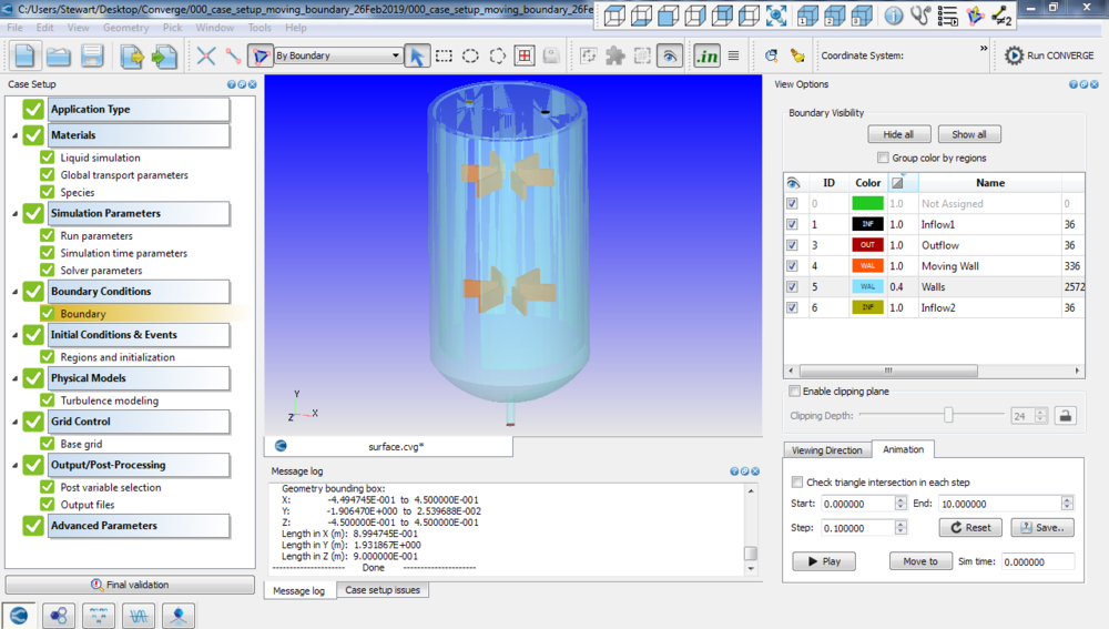
Task-Based Navigation system, which includes a sequential Navigation Bar and a dynamic Contextual Tool Palette
In general, the workflow for getting an analysis up and running within Fidelity is straightforward and intuitive, even for beginners without much training. The user interface features a file tree on the left, a properties window that pops up based on the file tree selection, and the main graphics window in the center. At the bottom-center of the graphics window, a very helpful “navigation” tool/work-flow widget displays the current stage/view of the project as well as the previous and future steps that must be marched through in order to run a study. The navigation widget is shown below and includes each step in a nice sequential fashion - Geometry, Domain, Mesh, Simulation, and Results. Just above the navigation workflow, a pie control panel shows available features/options that can be useful. The options in the pie control panel change depending on the active workflow step.

OMNIS User Interface and Flow Visualization
As the analyst steps through each stage of the progression, the geometry, mesh, etc. can be set up as needed, and you can jump back a step or two if something needs adjusting or if a setting was forgotten without losing any settings. Below, I’ll touch on each step briefly.
Geometry
The first step is to import the geometry for the analysis. We used Parasolid format for our testing, but it should be noted that native CAD package compatibility is included for software such as SOLIDWORKS and CATIA. In addition to importing geometry, this step in the navigation also allows the user to create primitive geometry shapes as well, primarily for mesh refinement zones, which can also be imported in the same fashion as the primary geometry. In the Fidelity environment, this step also includes automated "AutoSeal" tools to quickly close gaps and prepare "dirty" CAD for simulation. Adjusting/modifying the imported geometry can also be performed here.
Domain
The next step is “Domain,” during which the imported geometry is split into the required boundaries and physics boundary conditions will be assigned. Nothing fancy here, but the general step-wise progression in this manner allows the user to be task-focused while not getting lost in the weeds of an analysis setup.
Mesh

OMNIS Mesh example with Wall Layer Refinement
Once the geometry and domain are set, next up is meshing. Built into Fidelity CFD is the hexahedral-dominant HEXPRESS mesher. During our testing, the mesher felt robust and provided high quality elements as well as boundary layer refinement/inflation layers. The ability to refine via inserting a “refinement geometry” is very smooth and intuitive. Mesh analysis is also easy, as is the ability to adjust settings and remesh (remember, the user can go back to domain or geometry easily with a single mouse click without losing any settings). One feature that we particularly enjoyed was the mesh “preview,” which shows the surface mesh on the geometry in the real time as the user adjusts cell size settings in the properties panel. This allows the analyst to see visually what the final mesh may look like prior to running the more time-consuming meshing step. While HEXPRESS is traditionally hexahedral-dominant, the Fidelity platform now includes options for polyhedral mesh generation and export to optimize cell counts for the solver.
The image below shows a refinement zone we successfully inserted within the center of a pipe. Both were created externally and imported as separate Parasolid files.
Simulation
Once your mesh is successfully created, its time to determine the simulation settings. Here, the fluid type and properties along with boundary conditions and solver settings, including stopping criteria, are set up. This step is also very intuitive, however, for us, the stopping criteria was a bit unique compared to other software packages out there. We will touch on this later. Once the simulation is ready to run, it can be launched from within the GUI with the click of a button, and then the “Results Analysis” is available for “co-processing”. This feature is helpful because the user can monitor any post-processing scenes of fluid contours, vectors, etc. while the simulation is solving.
Since our original testing, the Fidelity environment has expanded significantly beyond basic single-phase flows. The platform now supports advanced physics including multiphase modeling (VOF and Lagrangian), conjugate heat transfer (CHT), and combustion. Furthermore, the integration of Lattice-Boltzmann and high-order solvers provides specialized tools for aeroacoustics and complex transient flows. Steady-state and transient options are available, as well as both laminar and turbulent models (K-Omega, K-Epsilon, Spalart-Allmaras, and others). This evolution fulfills Cadence’s goal of bringing a comprehensive suite of physics into the unified Fidelity environment.
Results Analysis
Once the simulation completes, the final step in the navigation panel work flow is Results Analysis. Here, the typical post-processing tools are available within the main GUI window, including making clip planes for contour/vector images, as well as line probes for data extraction. Creating “quantities” is a nice touch that allows the user to create custom values (at each cell) derived on solved continuum properties. One example available in Numeca’s user guide is to create a user vector field “momentum,” (the density times the velocity vector), which can then be plotted via a vector plot.
The Fidelity environment has matured significantly in this area, now including the advanced charting, streamline visualization, and automated report generation tools that were missing in early versions. These updates allow users to create detailed monitors and reports for field properties like velocity or density at specific locations or on defined planes. Furthermore, the ability to export scene images and high-fidelity animations during the solve is now natively supported, making it much easier to document transient simulations and share insights with non-technical stakeholders.
Other Points
We found that both setting up a case and getting it running were very intuitive. However, we found it challenging to balance computational expense and accuracy, as methods for determining convergence of simulations was atypical compared to other software packages. Typically, convergence of a simulation is measured by the minimization of the global numerical errors in solving the system of algebraic equations representing the discretized version of the relevant partial differential equations. As a steady-state simulation progresses, these “residuals” track to lower and lower values and the “error” in the solution is reduced. Generally, residual values are tracked per “iteration” of the numerical solver and a stopping criterion can be set such that the code is run until residuals reach a certain target value (such as 1.0E-4 or so). Within the Fidelity environment, though, such residuals are not handled as is typical.
First, residuals are not tracked via a normalized/averaged global error across all cells—they are tracked based on an order of magnitude basis in relation to the original solution. This means that instead of tracking towards a residual target of 1.0e-3 or 1.0e-4, the equivalent target is -3.0 or -4.0, corresponding to 3 or 4 orders of magnitude reduction in error from the initial iteration. In our original testing, getting down to this level for a simple laminar pipe flow case took an extreme amount of time on a multiple core machine; one tutorial failed to hit the convergence criteria in over 4 hours on 16 cores. However, the 2026 Fidelity platform is now optimized for Native GPU acceleration, which significantly overcomes the high computational cost previously seen on multi-core CPU machines.
The second thing we noticed is that these residuals are tracked every “cycle” and not “iteration.” To us, a cycle is a multigrid scheme term, as within each iteration of a multigrid algorithm, the matrix is coarsened and relaxed for several layers in order to solve the finest grid more efficiently. We did note that inputting the number of iterations as a stopping criteria does not necessarily end the simulation at that number of cycles. Since the solver uses a multigrid approach, the number of iterations input as a stopping criteria may be meant for the final/finest grid only. In the current Fidelity multigrid scheme, a cycle encompasses these multiple relaxations across coarsened grid levels, and Cadence has since improved its documentation to shed more light on independent multigrid residual tuning to limit this confusion.
The parallel processing seems to be working, however, our initial test cases took significantly longer to reach convergence versus other solvers. This could be due to the fact that the residual tolerance applies to all of the multigrids. In any case, more light should be shed on determining convergence through residual errors via user documentation. We did not originally test any batch mode processes or cloud computing; however, the Fidelity CFD platform is now fully integrated into cloud-native environments like Rescale, offering scalable, on-demand GPU resources for large-scale studies.
Licensing and Cost
Fidelity CFD is now available on the cloud. For Fidelity CFD, Cadence OnCloud is available starting at $2000/mo for 200 Tokens/mo. According to their website, a Cadence Token is a representative of computational usage giving you access to the tools you desire without the need for long-term contracts.
Summary
Cadence Fidelity CFD Suite (formerly Numeca OMNIS) is a solid, professional-grade tool that allows a wide range of users—from novices to experts—to efficiently set up and run complex analyses within a single environment. Since its initial release, the platform has fully integrated advanced physics capabilities from the legacy FINE product line, including robust multiphase modeling, moving mesh, and conjugate heat transfer. Post-processing has also matured significantly, now featuring automated report generation and high-fidelity visualization tools that rival other top-tier commercial products. With its massive GPU acceleration and unified workflow, Fidelity has successfully evolved into a comprehensive multiphysics platform.
Part 3 Conclusions:
All three of the tools discussed above have the potential to be extremely valuable in the right context. COMSOL brings unique capabilities for combining custom physics with pre-packaged solution methods for fluid dynamics. It also provides strong multi-physics capabilities and decent workflow, pre-processing and post-processing capabilities. Its drawbacks are its computational expense (memory and speed) due to its reliance on finite element methods and its cost when combining multiple modules to achieve expanded multi-physics. While newer 2026 releases have improved memory efficiency, the FEM-based overhead remains a factor for pure CFD.
Meanwhile, CONVERGE CFD possesses plenty of state-of-the-art tools to be used in simulating internal combustion engines and is quickly adding many capabilities for a wider range of applications, including electric motors and battery thermal management. Its unique approach to adaptive meshing will be of interest to any practitioner wishing to produce high fidelity results on micro-scales where regions requiring mesh refinement are not known prior to meshing. Its biggest drawback historically was a clunky workflow due to limitations on pre-processing and the requirement for a 3rd party post-processor; however, the current integration of ParaView Catalyst has significantly improved the in-situ post-processing experience. We also originally noted concern with the computational expense of remeshing at each time step on moving boundary problems.
Last but not least, Cadence Fidelity CFD (formerly Numeca OMNIS), which has since become the cornerstone of Cadence Fidelity CFD suite (following Cadence’s acquisition of Numeca in 2021) combines the excellent physics modeling capabilities of its diverse suite of software into an integrated workflow environment. While the original release was a bit rough around the edges with regards to the finer points and lacking any multi-physics capabilities, its workflow is smooth and pre- and post-processing are adequate. As of 2026, the "rough edges" have been smoothed out, and the platform has fully integrated the advanced multiphase and moving mesh physics from the legacy FINE product lines. We will definitely be keeping an eye on its future development.